In SQL, SELECT DISTINCT allows us to obtain only unique values from a list. What about Excel select distinct? How can we obtain unique values from a list dynamically with a formula? In this guide, we find out exactly that: a formula in excel to select distinct values dynamically. This guide is updated in 2021, and it simplifies a lot what you have to do with new formulas.
Excel Select Distinct (Quick and Easy, 2021)
Excel Select Distinct Formula (=UNIQUE)
This is the new method we should use, because it is literally just one formula to create our Excel select distinct result. The formula to select distinct values in Excel is Unique.
=UNIQUE(array, [by_col], [exactly_once])
It’s not an array formula in the strict sense, it is just a normal formula that you complete by pressing enter, just like SUM or any other normal formula. The parameters it wants are the following.
- Array – This is the list that contains all the value, out of which we want to extract only distinct or unique value
- by_col – True to select unique values within a column or vertical array (default), false to select unique values within a row or horizontal array
- exactly_once – True to perform an Excel select distinct and return each different value only once, false otherwise.
Now that you know the theory, let’s see it in practice because it is very simple.
Excel Select Distinct Example
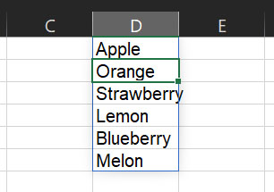
In the A1:A13 range we have a list of fruits, most of which are repeated. We want to extract a list containing each fruit exactly once, removing duplicates with a formula. For that, we resort to =UNIQUE, in its simplest form.
=UNIQUE(A1:A13)
We input this on a cell, D1, and it automatically fills the cells below as needed. This means we need to have enough space below the cells we are entering the UNIQUE formula to host all distinct values, otherwise we will get a #SPILL error.
If you select any cell in the range where you have your formula, you will see a shadow around all the cells that are auto filled with that formula.
To do that, we use the same formula, but we fill the last parameter as TRUE (or simply “1”). To fill the last parameter, we also need to input the optional parameter in the middle, which defaults to true, so we replicate the default value for that by specifying “true” manually.
Excel Select Distinct #SPILL Error
For the UNIQUE function to work and perform an Excel select distinct operation correctly, it needs to have enough space in the cells below it. With enough space, we mean enough space to present all the unique values, so how much space it depends on how much distinct values we have in the original dataset.
If, for some reason, we do not have enough space (we have some content below it), we will get a #SPILL error, meaning that the results would “spill out” of the space that we have available.
If we get the error, instead of displaying as many results as possible, Excel will just present the #SPILL error in the first cell and show no result. This is to prevent that we do some calculation or analysis on incomplete data, with the conviction of having the full set.
By selecting the cell with the #SPILL error we can see a border that shows where the results are to be plotted, so we know how much space we need to make for them.
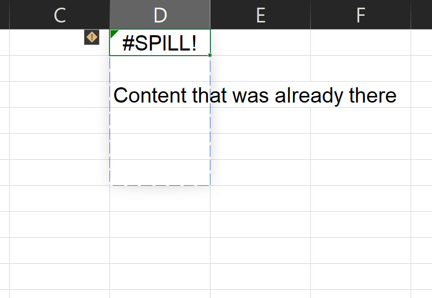
In this case, we can simply remove the previous content and the UNIQUE formula will go ahead and automatically fill the space that we make available. Yet, in other cases you may need to add additional rows or have content you cannot remove, thus you will need to do more advanced work to create the space you need.
Excel Select Distinct (Cumbersome, 2007)
This is the approach that you will find in many other tutorials online because it was the only one available until 2020. It involves an Array formula, a formula that returns multiple values and not just one.
Since this is an array formula, you cannot complete by pressing just Enter like a normal formula, but you complete it by pressing Ctrl + Shift + Enter. Furthermore, you do not select only one cell to see the magic fill the cells below. You have to select all the range where you want your results to appear, then enter the formula and then save it with Ctrl + Shift + Enter.
The idea is this simple: for each cell in the original dataset, we check if we already returned it up until now. If not, we return it, otherwise we just skip it.
For the American version of Excel, use:
=IFERROR(INDEX($A$2:$A$10, MATCH(0, COUNTIF($B$1:B1, $A$2:$A$10), 0)), "")
For the European version of Excel (with semicolons), use:
=IFERROR(INDEX($A$2:$A$10; MATCH(0; COUNTIF($B$1:B1; $A$2:$A$10); 0)); "")
Remember to complete it with Ctrl + Shift + Enter, otherwise it will not work!
In this formula, that we type in cell B2, we have two key parts:
$A$2:$A$10is the range of the original dataset, it must be fixed (with $ sign)$B$1:B1is the range of Excel select distinct values that we have obtained up until now. It starts with B1, which is the header and that must be different from any value in the list, and as we will go down the second part of the range (B1 without dollar sign) will move down to include more and more data, so we are able to check the data that already fetched.
It is crucial that you have a header, and that this header (the first line) contains a value that never appears among the list of values in the original dataset.
Excel Select Distinct in Summary
In short, using Excel to Select Distinct values is extremely easy now that we have the UNIQUE formula. We just need to input our original data set and that’s it. With this knowledge in mind, you can go on creating complex Excels and data models, in a way that is simply unprecedented.
If you want to know how to put your skills to good use in finance, I suggest starting with this ultimate guide on Net Present Value. You may also want to check Microsoft Excel official website.